
Starting with many of the same assumptions Munro used to model polarization in a worm cortex, we have created a computational simulation of morphogenesis in two dimensions. Here we describe a simplified version of our fully adhesive model. In this version, adhesion is not modeled directly; rather we focus on how differences in local cortical tension can generate morphogenetic movements. One advantage of the simplified model is that it runs much more quickly, a single simulation taking mere minutes on most computers. This means that systematic parameters searches for a wide range of conditions are feasible, and also makes it possible to rapidly explore the effects of a wider range of conditions such as starting geometry. The simple model is also suitable as a teaching tool, allowing rapid exploration of how variations in local tension affect the geometries and movements of groups of cells.
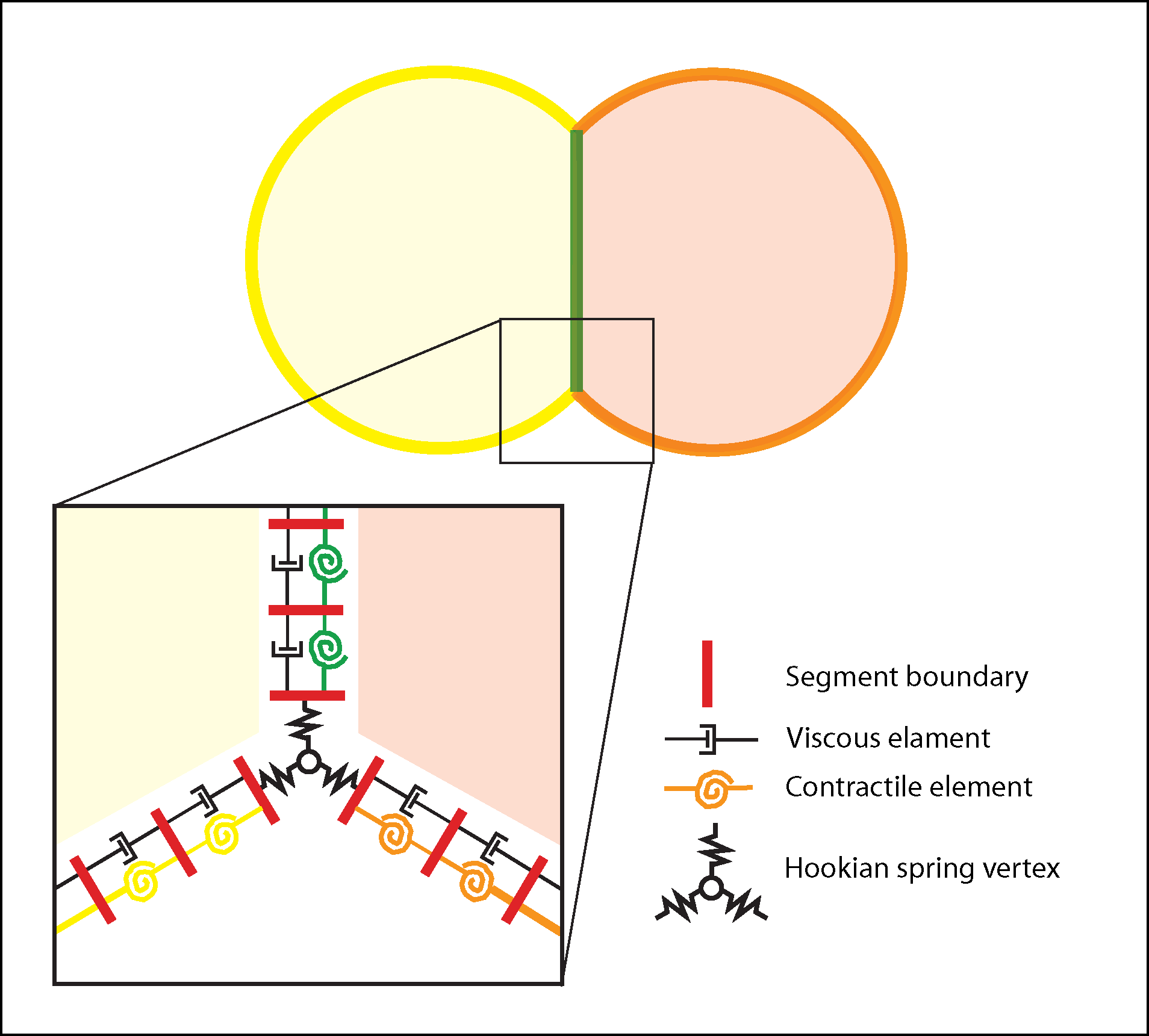
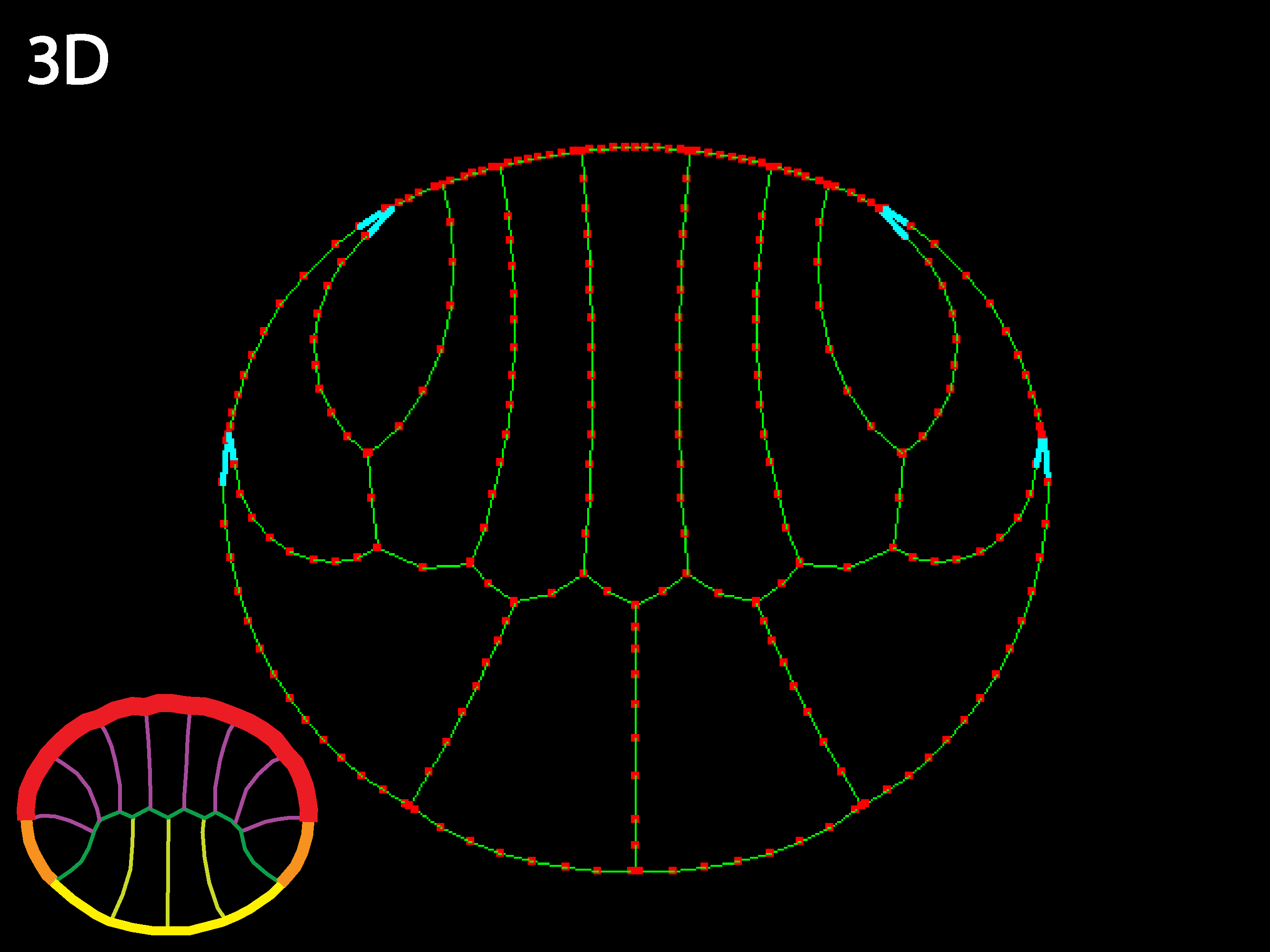
Conceptual basis for morphogenesis simulation. Starting conditions, specified by an input file called a netfile include cell number, type, areas, aspect ratios, locations of initial contacts, and local contractile tension. Tension can vary both with cell type and with apical (yellow/orange) or basolateral (green). In the tutorial examples below, the model cells represent a cross or sagittal section with apical outwards and basolateral interior, though they could equally represent a planar array of cells sectioned through their lateral regions. Cells maintain a nearly constant 2D “volume” (i.e., a hydrostatic pressure force counters attempts by forces to expand or contract cells); they are bounded by a belt of cortical segments with viscous and contractile elements in parallel; inner (basolateral) margins are a single, shared boundary between cells; vertices are points connected to the viscoelastic belts by stiff springs. Vertices and segments can rediscretize as needed to accommodate changing cell contacts, shrinkage or expansion, though the current version of code prevents cells from losing apical surface completely (i.e. ingression is not allowed). A collision detector (whose action shows up as cyan lines in the simulation output) prevents overlapping of cells. In the output of the simulation, red squares mark borders of green cortical segments, and their movements indicate cortical flow.
The examples shown below demonstrate, first for a pair of cells and then for a cross-section representing an ascidian embryo, how local differences in contractile tension affect the shapes that cells and embryos adopt under simple conditions (no growth, cleavage, protrusive activity, or microtubule-driven shape changes). Following the examples, we explain how to download the code, run simulations, and modify input files to create particular starting conditions. Because we are currently preparing the initials papers based on this code for publication, the source code is not yet available for download.
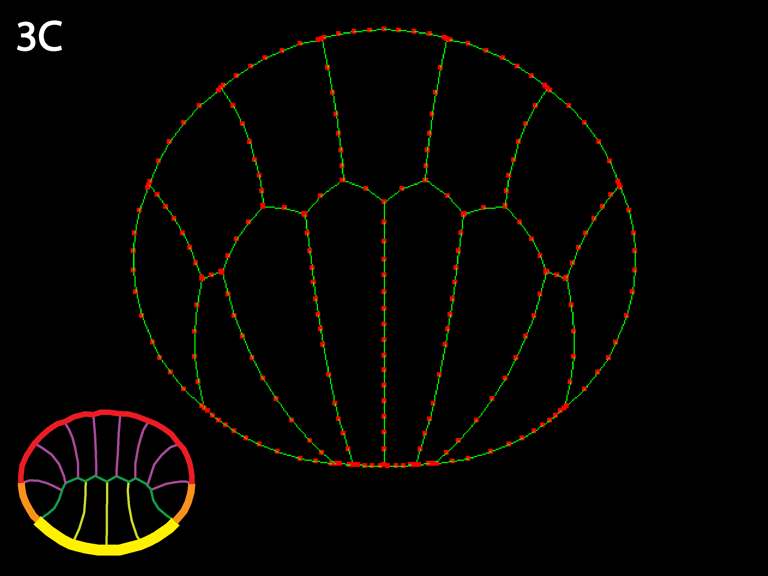
For the following examples, the icon in the bottom left of each corresponding picture shows the relative local contractile tensions, with thicker lines representing greater tension. The figure shows the equilibrium state for each simulation; click on the figure to see simulation movies.
Note how the initial rectangular geometry is rapidly converted to realistic curved shape by the action of contractile tension against nearly incompressible cells. This greatly simplifies the specification of input geometries, which can be confined to rectangles and triangles for most cases.
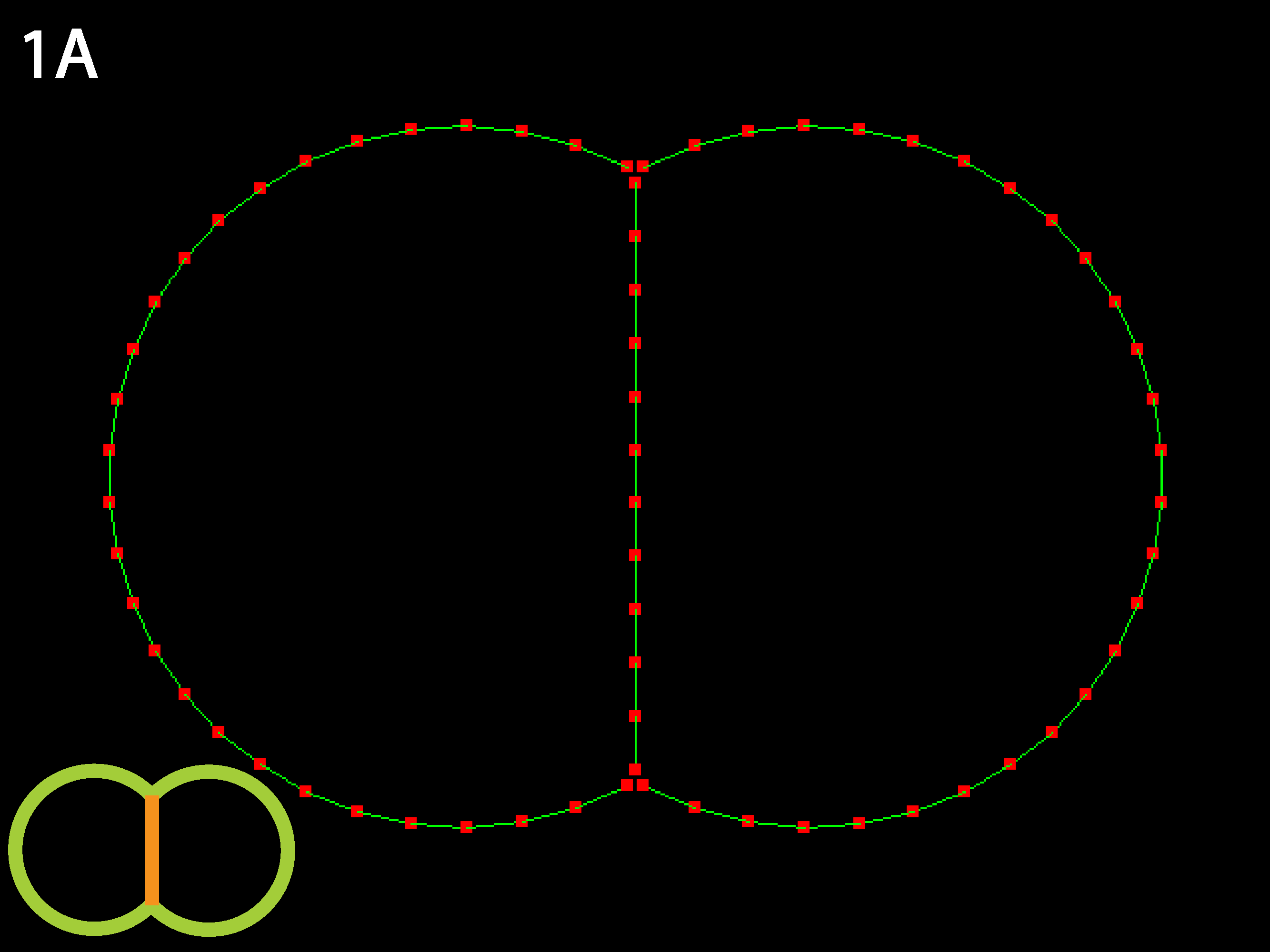
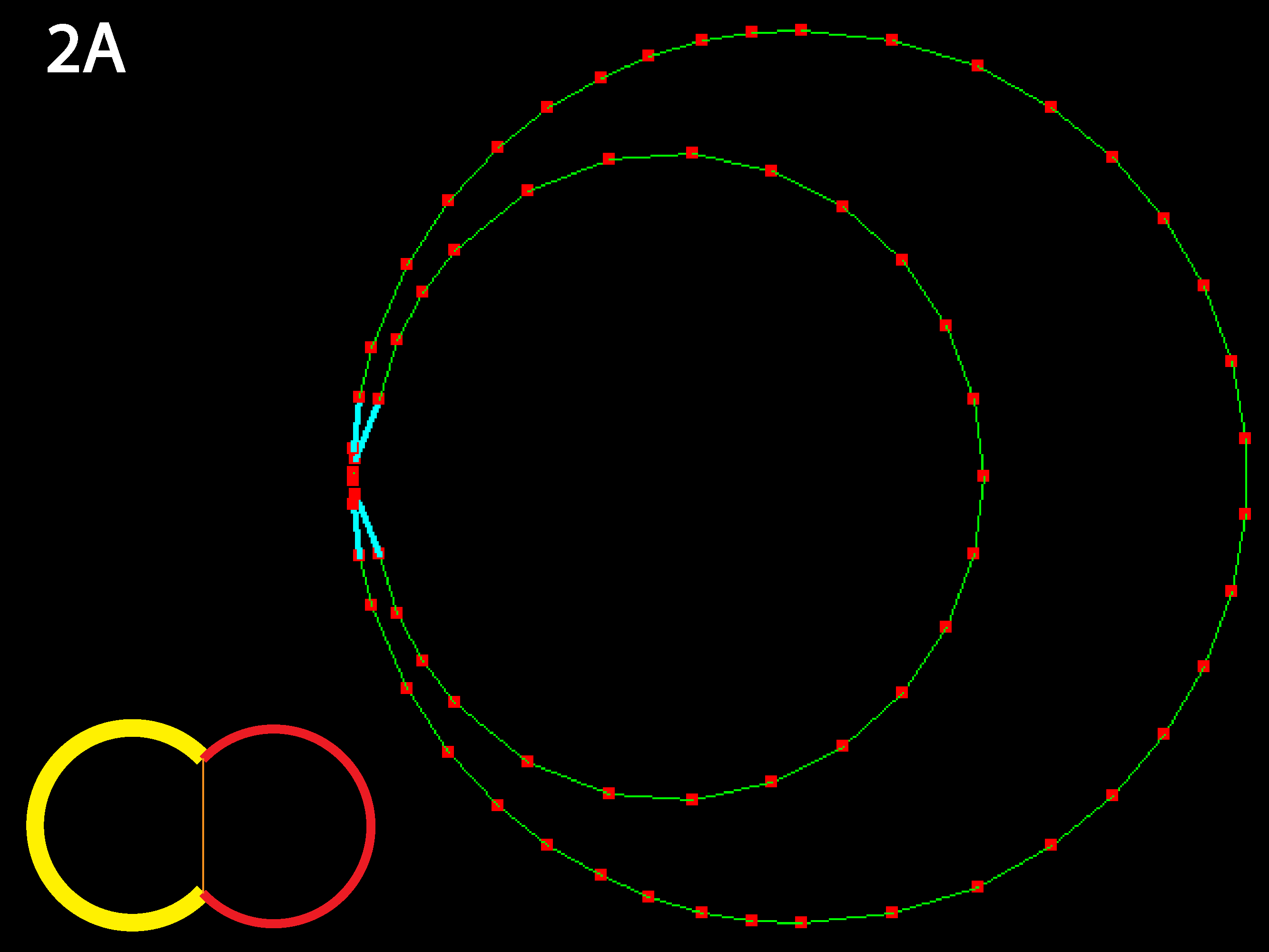
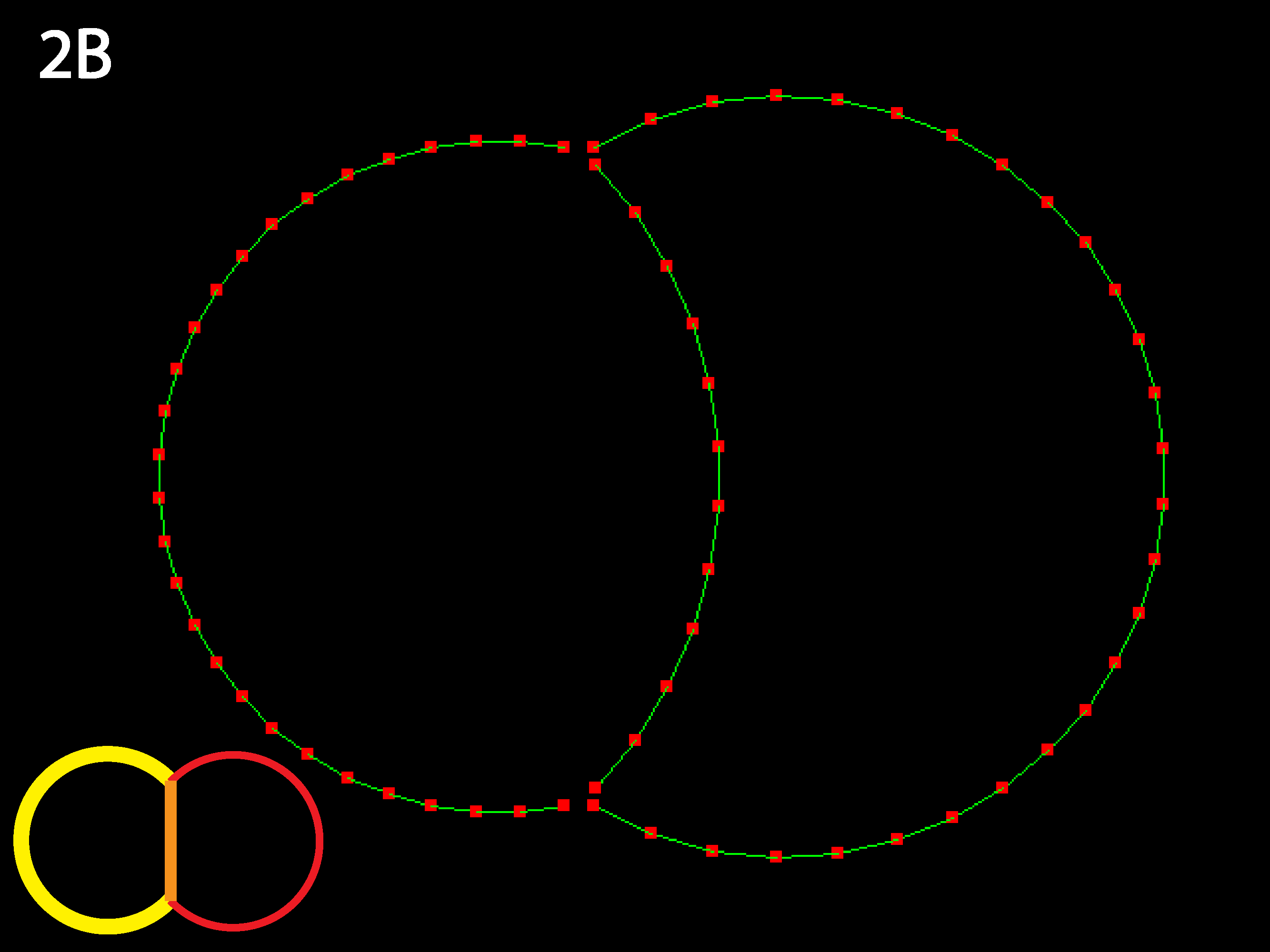
Equilibrium is two round cells with substantial contact with each other. Because relative rather than absolute parameter values are determine the equilibrium state, raising or lowering the tension uniformly (see Running Simulations below) will only affect time to equilibrium, not the equilibrium shape.
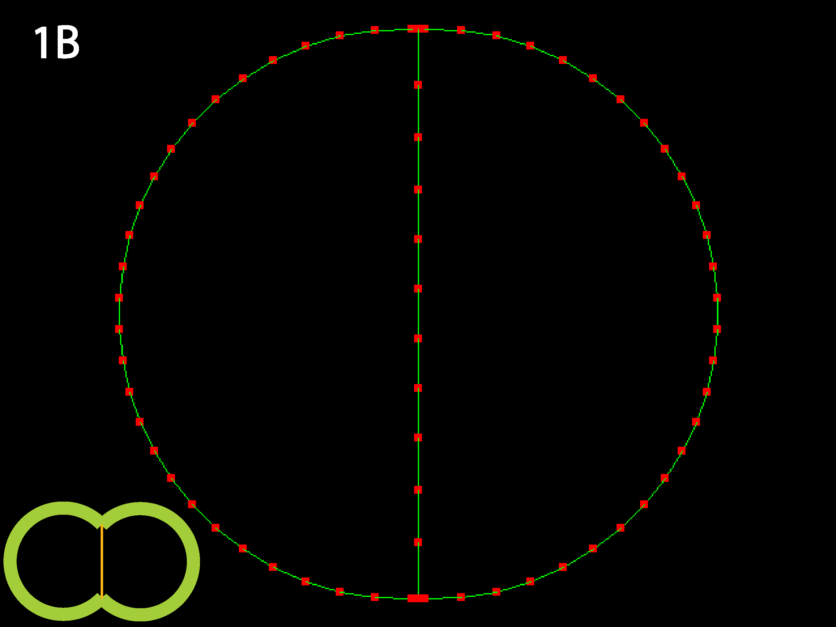
Outer tensions dominate and cells minimize their outer margins, meaning individual cell shapes must accommodate this tendency for giobal isodiametry (see below 3B for similar case with multiple cells). Because in this code adhesive behavior is folded into inner tension values, a decrease in relative inner tension can also be viewed as an increase in adhesive strength, and the converse (as shown in 1C directly below).
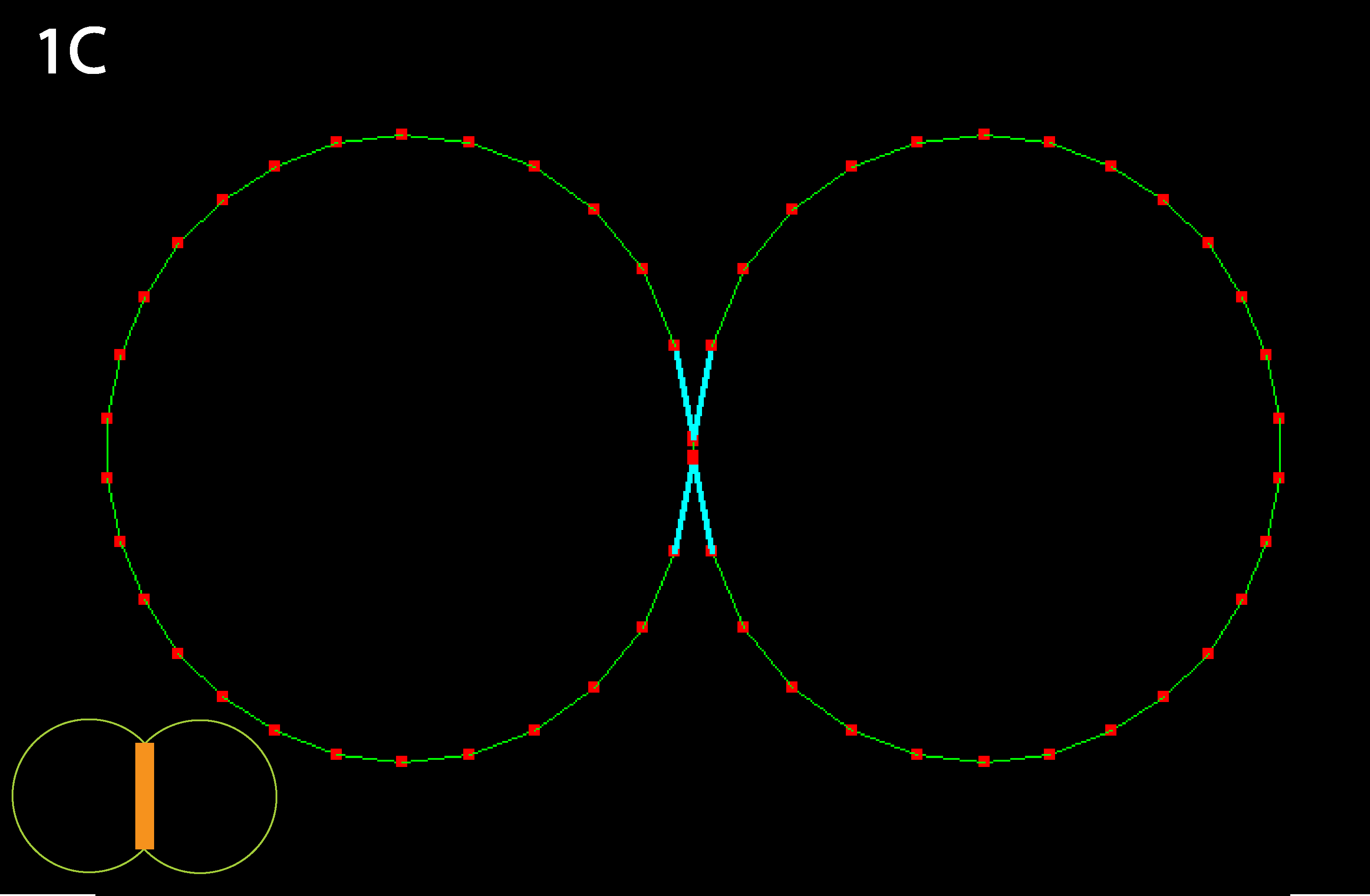
Inner junction constricts to the point that cells detach; as mentioned in 1B this could alternately be viewed as the result of a decrease in cell-cell adhesion, as occurs in calcium-free medium (note: cyan lines indicate that a collision detector is acting to prevent illegal overlapping of cells). Note that in real cells, inner tension is usually less than outer tension, as indicated by reduced basolateral staining for actively contractile myosin.
The RC apical zone shrinks to almost 0. For less extreme differences, equilibrium is the same but takes longer to reach. The code as written prevents apical junctions from shrinking to 0, though it permits inner junctions to do so making neighbor exchanges possible.
Now the RC apical region is prevented from shrinking to nearly nothing as its contractility is sufficiently balanced by the strong inner tension. Try varying these three parameters to discover the boundaries of different equilbria (see Running Simulations section below).
Three cell types (outlined in icons at lower right), endoderm yellow, ectoderm red and mesoderm orange. Ascidians have almost no blastocoel and the blastula stage in cross or sagittal section appears as two rows of cells, forming the animal (the ectoderm) and the vegetal (endoderm and mesoderm) hemispheres. Note that the simulation code download available here could accommodate embryos with large blastocoels and a lack of basal cell contacts by simply adding a new cell type called “Blastocoel” to a new netfile (see Creating/modifying Netfiles section below). Simulations will, however, run slower as the number of cells and cell types increases and as the need for shorter timesteps or more stringent collision detection increases as may occur for certain geometries, e.g. those with very skinny cells.
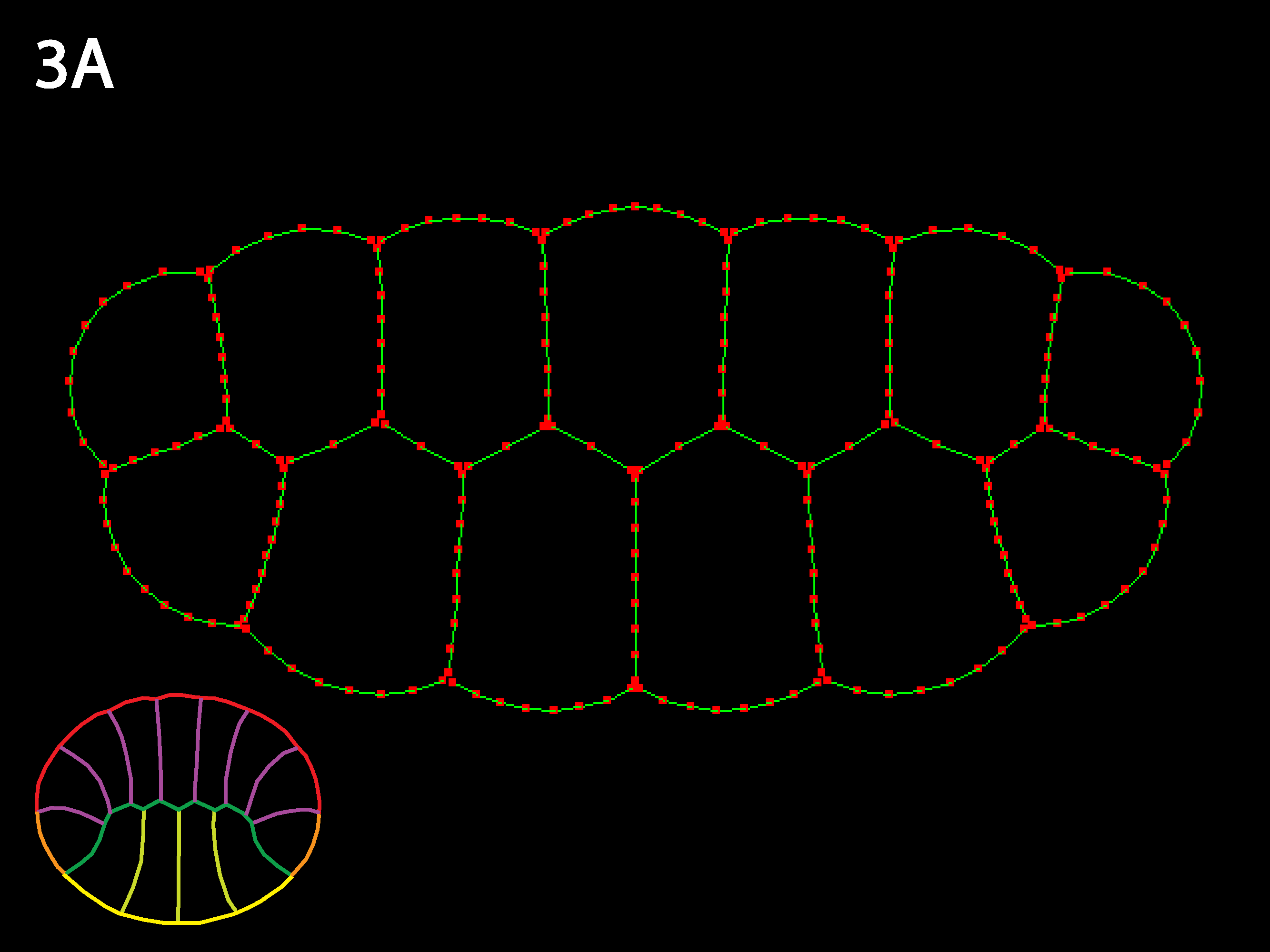
Similar to 1A: because inner tensions are as high as outer, the individual cell shapes remain close to isodiametric and the 2-row embryo shape changes little. As values of inner tension approach outer tension, individual geometry (shape, size, and initial arrangement of cells) is much more important in determining embryo shape—e.g. for double row, double row continues to exist or even gets more prominent. The embryo is like a union with very strong individual states.
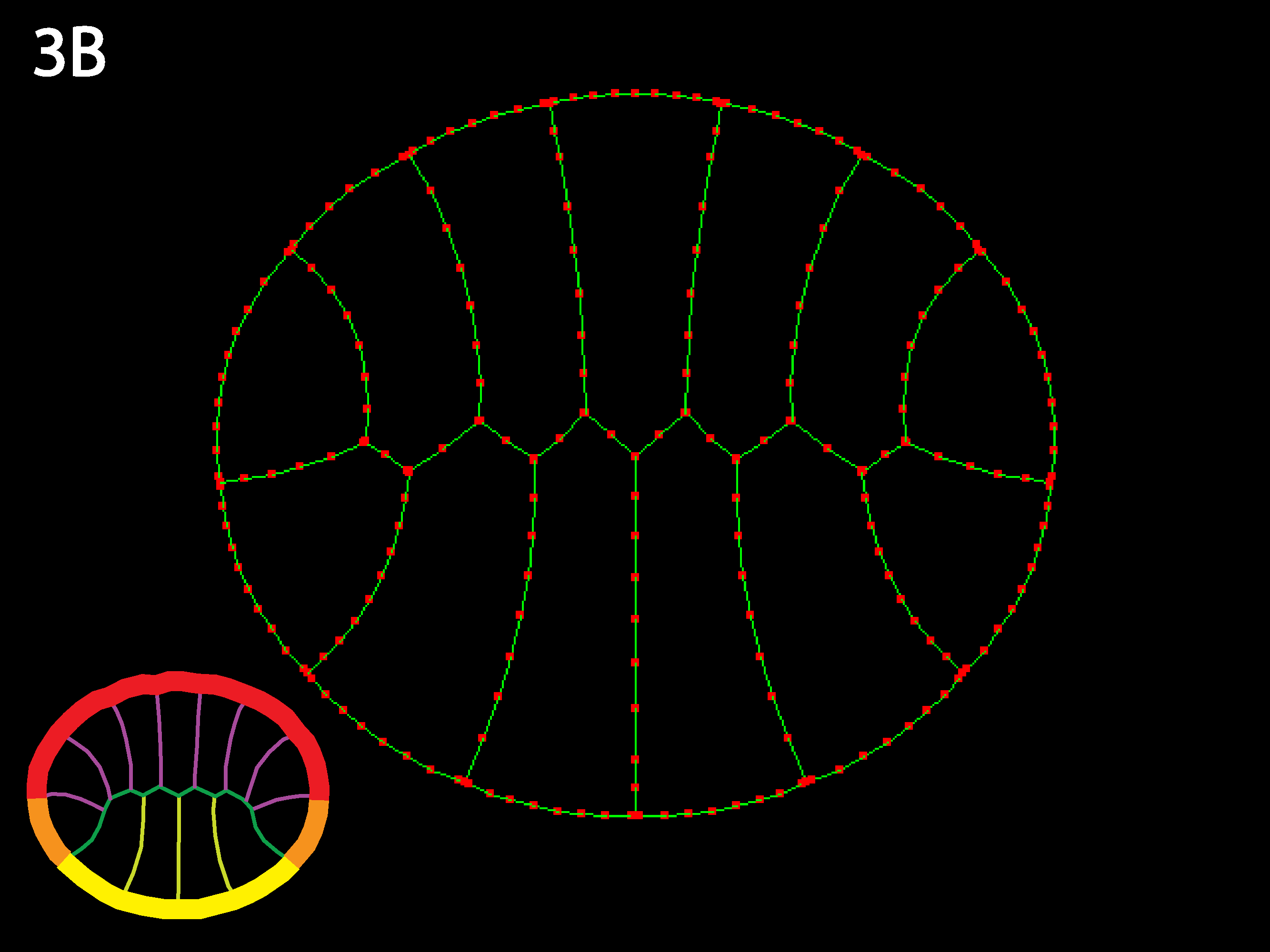
As in 1B, the strong outer tensions attempt to form the embryo into a circle, deforming individual cells to do so. In contrast to 3A, when outer tension dominates, individual geometry less important—global forces make embryo want to be round regardless, and individual cells get as deformed as necessary to accommodate this. The embryo is like a union with very weak individual states.
The situation gets more complex and interesting when cells are allowed to differ from one another, as is of course a prerequisite for morphogenesis.
This is a simulation of apical constriction. Note that apical constriction does not invariably cause invagination, but the context in which it acts (arrangement and mechanical behavior and responses of surrounding cells) helps determine the outcome. In this example, although cells shrink apically they also lengthen substantially and do not form an invagination. Note how the edge cells get stretched into crescents (in fact quite similar to what we see in cells at the edges of the animal and vegetal hemispheres in ascidian embryos).
Note that the example embryo is asymmetric top to bottom in both cell shapes and in distribution of types (there are only 4 endoderm but 7 ectoderm—see icon color-coding). Reversing the cells relative outer tensions reveals how sensitive the simulation is to variations in initial geometry—the initially narrower ectoderm apices contract more strongly and the initially wider endoderm apices spread more than in 3C.
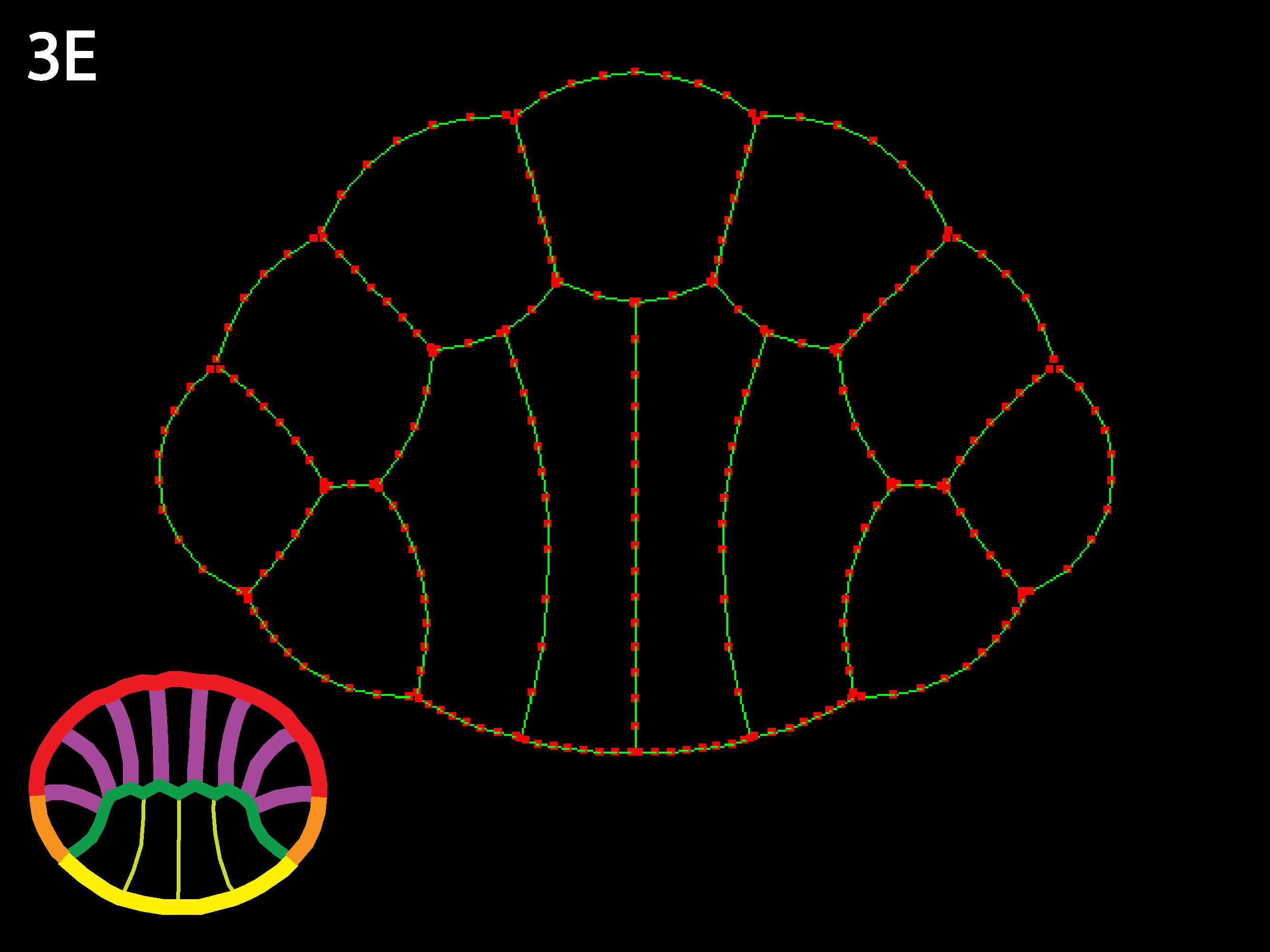
Allowing inner tension to vary locally with cell type also generates interesting shape changes, such as columnarizations and shortenings. In a real embryo, active shortening of inner boundaries of cells could only columnarize cells basal to them if they were strongly attached basally, which would not necessarily be the case, though other constraints and transmission of forces through the embryo could also allow some columnarization under these conditions.
Many other combinations of local tension values are possible and can be explored by downloading the simulation and modifiyingn the parameters in the user interface (see below). If the user wishes further to create their own initial starting geometries with varying numbers of cell types, see Creating/modifying Netfiles below.
Download the MorphogenesisSimulation folder containing cortex.jar and two .net files. You will need Java to run this code. Mac OS X users already have java; PC users will need to download and install java if it is not already installed.
To start the code, open a terminal window and navigate to the directory containing the cortex.jar file (e.g. by typing
"cd ~/desktop/MorphgenesisSimulation”
if the folder is on your desktop). Then type the command
"java -jar cortex.jar”.
The simulation should open after a moment; the initial picture is one rectangle which won’t do much, morphogenesis-wise. Under the File menu select “Open Model” and select a netfile from the MorhpogenesisSimulation folder. You should see some rectangles appear in the window.
To start a run, select Run-> Run. To pause a run (if you wish to change parameter values, for example), select Run -> Pause Simulation. If you wish to load a new netfile you will have to kill the simulation first (Run -> Kill Simulation). For mysterious reasons they sometimes have to be killed twice.
The buttons on the lower section of the window are used to navigate through the simulation output frames. On the left, the arrows move the image and the center ellipse centers it. The small and large squares increase or decrease size of the red squares marking cortical segment boundaries, the next three buttons set magnification (ellipse returns it to original setting). The set to the far right lets you move through the frames. If memory is low, these buttons may not appear but are still clickable.
If you wish to change parameters before starting the simulations, select Window-> ShowParameters. Parameters can also be changed during a simulation run, either after pausing it or on the fly. The tension parameters are at the end of the list, under Affectors. Many of the other parameters either are not relevant to this version of the morphogenesis code or may cause serious trouble with simulations if they are changed too much, because their relative values have been tuned to both mimic real cells and to allow for smooth running of the code’s calculations. Parameters that may be of interest to modify, besides cortical tensions, include under (Cell Mechanics) fRepulse (strength of collision detector—may need to be increased for some situations; cyan lines in simulation output indicate that collision detector is acting); note that the innerT and outerT listed here are default values and do not affect cell types defined in a netfile; and (under Integration Control) min and max SegLength (affects discretization of cortex), tStop (how long a simulation will run for), dtStep (length of a timestep), and iFramesSave (how often frames are saved). Note that some of the other menu choices are designed for use with iterated code runs, and so are not described in this tutorial.
To restore default values to parameters, just open the model again.
The input file (called a netfile) specifies a simulation’s initial geometry (cell numbers, sizes, contacts, aspect ratios—for simplicity we typically use rectangles and triangles, which cortical contractility rapidly reforms to appropriate cell shapes), number and arrangement of particular cell types (whose mechanical properties are to be distinguished), and initial values for cortical tension parameters. These and other parameters can be also be modified in the user interface (parameters window) when a simulation is initiated or while it is running.
The example netfile, which corresponds to figure 1 and was used to generate examples 1-2 above, specifies two cells of equal volume but different type, allowing unique inner and outer tension parameters to be specified. Each cell has a long outer junction (apical surface) and shares an inner (basolateral) junctions with its neighbor.
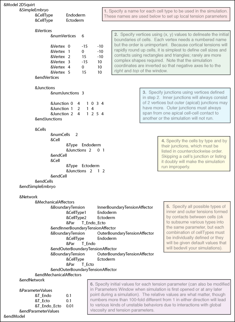
When making modifications to this template, there are several common pitfalls to be avoided. The number of vertices (numVertices) must match the actual number specified, likewise for numJunctions and numCells. If a new cell type is added its inner and outer tension parameters must be specified as needed; otherwise a default tension value will operate and may cause problems. For example, if there is only one mesoderm, or they will never touch each other, there is no need to specify a T_meso_meso. If you wish to subsume one category into another, e.g. T_endo_endo to be the same as T_endo_ecto, you may give them a single name such as T_endo_any, but both variants much be specified. Other common problems with netfiles involve overlapping junctions or impossible geometries—carefully sketching out the embryo map, or making changes one a time to a working file, is the best way to avoid these. Finally, typos will cause hard-to-notice bugs—if you misspell a cell type, the code will still run but that cell will receive default, not desired, tension values. The netfile can be edited in programs such as SimpleText, but will need to have the tag .net to be recognized by the simulation code.
Although the code can deal with 4-way vertices, simulations run more realistically if cells are limited to 3-way vertices (as most real cells are, except during brief transitions). In practice, to represent a particular embryo geometry can require a good deal of trial and error to balance the need to generate accurate cell-cell contacts, aspect ratios, volumes, and numbers. Often a special set of initialization tension parameters, run for a specified length of time, can help generate the desired geometry as well.
Here is an example 13Cell3Types.net of a netfile for a more complex geometry, representing the cross-section of an ascidian blastula just before gastrulation begins and used to generate simulations shown in figures 3A-3C above. There are four endoderm cells, which will be on the bottom when the simulation opens, two flanking mesoderm cells, and the rest ectoderm. By varying the outer and inner tension values for the different cell types, many interesting transformations can be achieved, including placode formation and invagination. By varying starting geometries and contacts as well, the user can gain a sense for how locally modulated cortical tension can shape cells and embryos.